|
bp |
|
|
|||||||||||||||||||||||||||||||||||||||||||||||||||||||
|
Corporation Number # 629729-3 |
|
We are specialized in quality, innovated product, modelling, simulation, operation, equipment and service. Head
office: North America +1(519) 893–5852 |
|||||||||||||||||||||||||||||||||||||||||||||||||||||||
|
Homepage
About Us Q/C
Division |
|||||||||||||||||||||||||||||||||||||||||||||||||||||||||
|
ut
Here you may get yourself round certain corner of whole picture. [ For design, consult, ... please contact us.]
Computational
Fluid Dynamic [CFD]- useful Materials: pros and cons between Reynolds-averaged Navier stocks (RANS) and direct numerical simulation (DNS) modeling. Solution: DNS solves the Navier-stocks equations in their original form without time averaging or further modeling of turbulence. Since even turbulent flows satisfy the N-S equations, this will give an exact solution, which includes all turbulent scales. However, an extremely fine mesh must be used in order to resolve the finest turbulent length scales. This requires prohibitive amounts of computational power even for low Reynolds numbers (#CV=Re ^9/4). DNS is therefore not currently suitable for most flows of engineering interest. RANS models turbulence in the N-s equations by applying a time average to all turbulent fluctuations. The resulting Reynolds tress terms are then approximated using various methods i.e. eddy viscosity, RSTM. The advantage is that turbulent effects are incorporated into the solution without the need for an extremely fine grid. RANS is practical for many engineering flows where DNS is too computationally expensive. The disadvantage with RANS is that turbulence must be modeled, not solved directly, which leads to approximation errors in the turbulence terms, more advanced turbulence models may be used (e.g. RSM, ASM) to reduce these errors, but with higher computational requirements.
the Major difference between mixing length and k-ε models. Both models use the eddy viscosity concept to model the turbulent viscosity, which in turn is used to calculate the Reynolds stresses. The mixing length model is a zero equation model, which expresses μt as a simple function of position within the flow. The function is based on analysis of simple flows and required the turbulent boundary layer thickness δ to be known. For more complex flow geometries, δ is hard to predict. The more general k-ε model can be used to find μt in terms of production and dissipation of turbulent kinetic energy. These two-equation models introduce two additional transport equations for k and ε, which are solved to give values of k, ε and μt throughout the flow. (μt = ρ.Cμ .k^2 / ε) Major difference: · Can be defined as definition of velocity and length scales and kinematic turbulent viscosity · Strong connection between the mean flow and the behavior of the largest eddies is the condition for attempting to link the characteristic velocity scale of the eddies with the mean flow properties. · Neglecting of Convection and diffusion of turbulence properties is the condition for k-ε model to express the influence of turbulence on the mean flow in terms of the mixing length. · How μt is calculated; simple algebraic function vs. two partial differential transport equations
Reference : H.K Versteeg, w. malala sekera. An introduction to CFD: the finite volume method . 1995. ISBN 0582218845 ************************************************************************************************************************************************************** Additional focused aspects a) Simulate compressible flow (Air) through a long plane square duct. b) Learn and practice basic CFX-built and CFX-TASCflow commends. c) Comparing drop pressure with analytical method (using moody diagram).
1 Summary The overall objective of this project is to simulate the developing turbulent flow of air in one quarter of square duct by using TASCflow professional software as CFX-Built and CFX-TASCflow for following purpose: · Using geometry development · Domain the region form. · Surface mesh seeding and generation. · Mesh spacing (increase, decrease). · Boundary surface identification. · Postprocessing and generate velocity and pressure in flow field. · Practice different boundary condition and how simulation be affected by upstream flow. · Comparison of results with analytical method moody diagram.
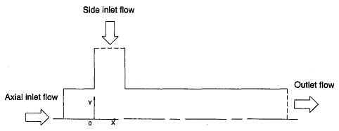
2 Purpose Definitions The developing turbulent flow of air in a duct is to be simulated. The duct is 0.5[m] square and is 30.0[m] long. All duct walls are smooth [WALLTR]. The working fluid is air with a density of 1.0[kg/m3] and a dynamic viscosity of 1.0E-5[kg/m-s]. The air enters the duct with an axial velocity of 2.0[m/s], turbulent kinetic energy intensity of 2%, and a turbulent length scale of 0.02[m] [INLET]. The inlet profiles can be assumed to be uniform. The fluid leaves the pipe at a uniform pressure of 0.0[Pa](gauge) [OUTLET]. All mean flow conditions are steady.
The solution domain should include the region from the duct centreline to the upper and rear duct walls. Use a relatively coarse mesh with the following specifications:
Number of nodes in flow direction =Ni+1 =15 → Number of elements=14 Expansion Factor in flow direction =1.1→L2/L1= (1.1) ^Ni-1, Ni-1 = 13 → L2/L1 = 3.45 Number of nodes in across the duct (half-height) = Ni+1 = 10 → Number of elements = 9 Expansion Factor in flow direction =0.85 →L2/L1= (0.85) ^Ni-1, Ni-1 = 8 → L2/L1 = 0.272 Number of nodes in across the duct (half-width) = Ni+1 = 10 → Number of elements = 9 Expansion Factor in flow direction =0.85 →L2/L1= (0.85) ^Ni-1, Ni-1 = 8 → L2/L1 = 0.272
A timestep appropriate to the global scale of the problem (i.e. the time for an average fluid parcel to move across the flow domain) should be chosen. Time step=30% of L domain/u inlet = 0.3*(30[m]/2.0[m/s]) = 4.5 [s] Convergence should be achieved within 40 timesteps with a maximum normalized residual less than 1.0E-4.
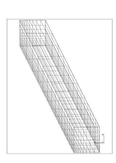
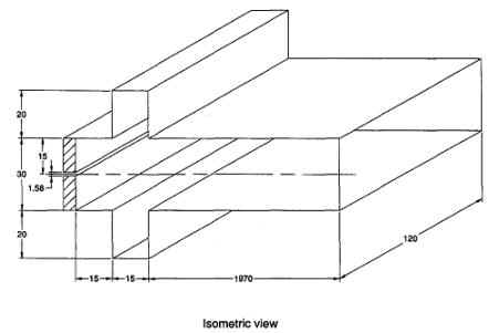
Figure 1. Setup for duct simulation 1-Whole duct
Figure 2. Setup for duct simulation_ One quarter
3 Simulation Setup
Figures 1&2 outlines the setup for this simulation. The co-ordinate system is defined with the y-axis aligned with the centreline of the duct with x=0 located at the inlet plane. Because of the twin symmetry of the flow, a one-quarter section of the duct is chosen (top right quarter) extending from the centreline to the top and rear walls. This choice of domain reduces the number of computational volumes by one quarter, which will reduce the total solution time required. The choice of appropriate symmetry boundary conditions along the front and bottom faces of the flow domain will ensure that the solution for the quarter section will apply to the full duct volume.
The node definitions provided above define a relatively coarse grid appropriate to this problem. Bias along the axial flow direction chosen because the expected flow field varies more near the duct inlet compared to the outlet. Similarly, the bias along the two transverse axes is chosen to concentrate nodes closer to the duct walls because this is where the flow field varies most due to wall effects The use of smaller nodes closer to the duct walls ensures that the boundary layer is properly resolved in the final results and increases the chances that the solution will converge.
Figure 5 shows the grid definition for this simulation including detail of the one-way bias meshes applied to the transverse flow axes. The surface geometry and grid were both defined in CFX-BUILD 4.
Summary of operating condition:
Length of duct =30 m Wide = high = 0.5 m
Air den=1.0kg/m^3
Dynamic viscosity=1.0*10^-5 kg/m/s Turbulent kinetic energy intensity= 2%
Maximum normalized residual <=1.0*10^-4 Convergence = within 40 time steps
Re Number =V.D.ρ/μ = V.D/υ 1.0[kg/m3]*2.0[m/s]*.5[m]/1.0E-05[kg/m/s]=100,000 → We should select HIGH Re Number
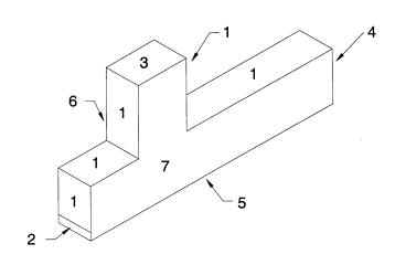
Figure 3. Approach to build a Surface (1) from a curve (1) by extruding in y-D
Figure 4. Approach to build a Solid (1) from a Surface (1) by extruding in z-D
Figure 5. Grid for duct simulation Figure 6. Nodes distribution along the duct axis Build geometry: · Collect a point as origin: as cross point (figure 3) · Generate point #1 [0.25,0,0.25] as starting point: point 1 (figure 3) · Generate point #2 [0.5,0,0.25]: point 2 (figure 3) · Create a curve between point #1 & point #2: curve 1 (figure 3) · Extrude curve in y direction <0 30 0> to make a surface: surface 1 (figure 3) · Extrude surface in z direction<0 0 0.25> to make a solid: solid 1 (figure 3) Surface mesh seeding and generation and boundary surface identification: · Choose boundary condition as (figure 2): Inflow: Inlet Outflow: Outlet Symmetry: West & South sides Wall: North & East sides
· Plot of grid, generate mesh seed in flow, cross flow direction, and apply mesh spacing based on expansion factor = ef and L2/L1 = (ef)^ (Ni-1) (figure 6) · Data entry for given data, identifying boundary condition, and focus on centre line [1,1:15,1] regarding variation of pressure along the axial flow direction (figure 4) Once the grid has been defined, boundary conditions appropriate to the problem can be defined. Figure 2 shows which boundary conditions are specified for this simulation; these conditions are summarized in Table A. The inlet and outlet conditions are defined according to the problem specifications above and are applied as steady, uniform profiles. The top and rear wall of the duct are modelled as applied as steady, uniform profiles. Finally, the behind and bottom boundaries of the flow domain are defined as symmetry surface, ensuring that no mass transfer or velocity gradient is present across either Table A
4 Simulation solution
Prior to solving this simulation, an initial flow field was generated using TASCflow. A value of U = 2.0[m/s] was set at all nodes and the same turbulent flow parameters were used as had been specified at the inlet. An initial guess for the flow field, which is reasonable close to, the final solution will help the simulation solve more quickly. In this problem it is reasonable to guess that the final flow field will resemble a uniform axial flow through the duct. The duct simulation was solved using TASCFlow 2.10. The solution parameters given above were used to set the total number of timesteps and the maximum allowable normalized residual. These parameters limit the amount of computational time invested in the solving the simulation. The timestep used was calculated based on 30% of the average residency time of a fluid particle in the flow domain: tstep = 0.30 (Ldomain/uinlet) = 0.30 (30[m] / 2.0[m/s]) = 0.30 (15[s]) = 4.5[s]
Note that this is a rough approximation used to choose an appropriate timestep to achieve a converged solution in a reasonable amount of time. Other larger timesteps could be chosen which may generate a solution in less time while maintaining convergence. The solution of this simulation took 34 steps for a total computational time. The maximum normalized residual was less than the specified level.
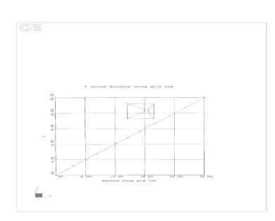
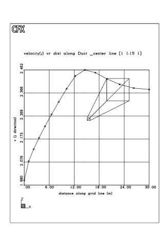
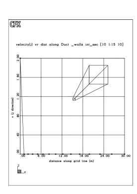
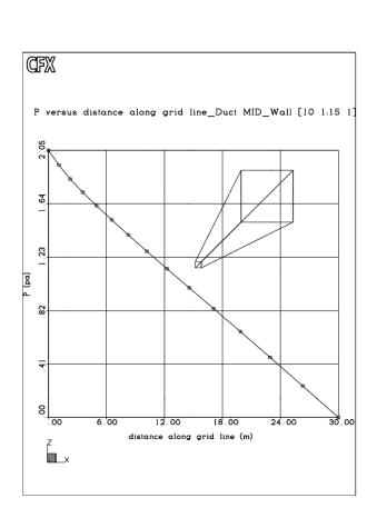
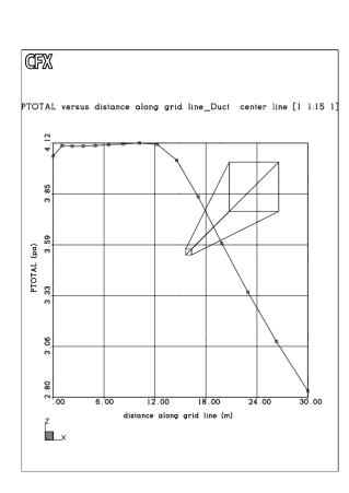
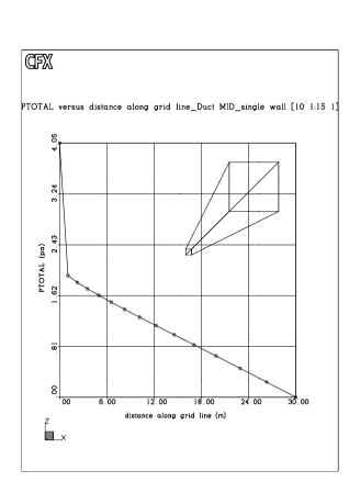
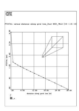
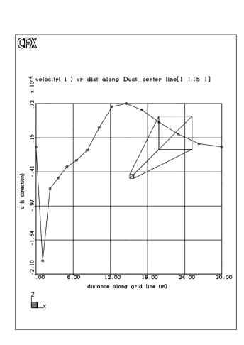
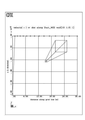
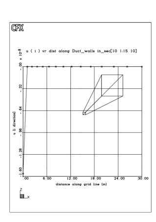
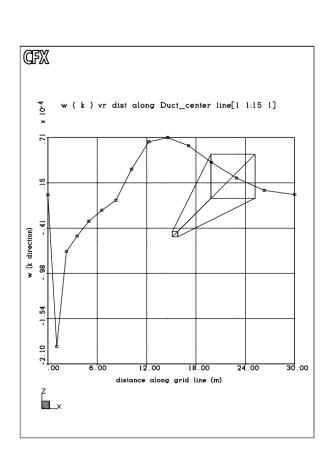
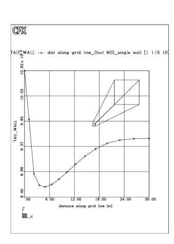
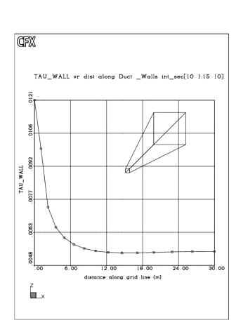
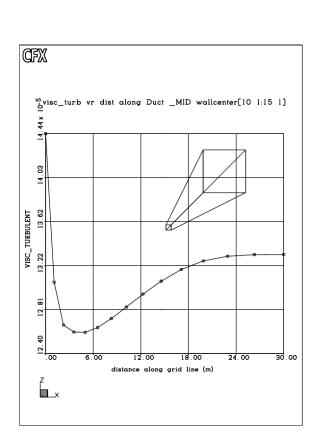
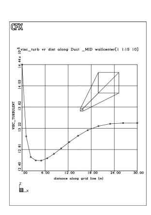
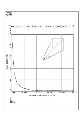
Figure 6. Flow velocity distribution along the duct in different Location- V (j-D) Note that the velocity close to the duct walls is very low due to high U (i-D) Note (in figure 4): Regarding variation of pressure node #1 to node #7 is non-linear; we conclude that the flow doesn’t develop at the beginning of duct that is clear when the flow builds up (at node #7,…) variation of pressure should be linear. Analytical results and predict drop pressure via moody diagram:
Diameter for non-circular duct = Dh
= 2ab/(a+b)
a
b
Table A
Reynolds
number = Re =
Moody
diagram
Illustrates the comparison of the calculated drop pressure and simulation results:The reason for differences between defined result from simulation and analytical method (moody diagram) can be specified as follows: · Number of nodes, grid refinement is the main tool at the disposal of CFD for improvement of accuracy of a simulation · Assuming duct walls are smooth which can shift result to farther and higher from analytical method · Expansion factor, which by decreasing and increasing the number of nodes results would be closed to real condition · Our simulation are effected by upstream (UDS) flow and Peclet number effect; Pe=F/D F=ρ.v =1*2=2 D=Г/δx = 1.0*10^-5[kg/m/s] / δx Which along the duct Pe number increases with respect to reduction of grid refinement and across the duct Pe number decreases with respect to grid refinement · UDS method has 1st order accuracy and content truncational error · Calculate timesteps · The applied accuracy in this simulation as maximum normalized residual is chosen as 1.0*10^-4 which itself can affect diversion · Moody diagram is specified for round pipe only with %15 accuracy · Moody diagram has less accuracy for other shapes, which are far from circle or round pipes · In this problem the faces e and w of the general nodes may not be at the mid-points between nodes E and P, and nodes W and P, respectively. That is why, the interface values of diffusion coefficients may vary.
Conclusion: · Although CFD code has a lot of weakness and conversion (about 20%) but still is very strong and powerful program which can demonstrate simulation and illustrate study of all kinds of fluid flow · Upwind (or upstream) fluid flow can affect on result of study and in particular, special care was given to documenting the flow at an upstream section so realistic initial boundary condition could be provide for computational studies. · CFD’s study provide sufficient information for anther worker
References: · Fundamentals of Fluid Mechanics, Third Edition, Munson, Young, Okishi. · Fluid Power Control System, Fifth edition, Anthony Esposito. · Data for Validation of CFD Codes, Vol.146, D. Goldstein, D. Hughes, R. Johnson, D. Lankford.
5 Results Figure 4 shows the results from the duct simulation. Note that the velocity and pressure gradients close to the duct walls are high and justify the mesh biases chosen in the setup. Figure 4. Speed countours for duct simulation. In order to assess the accuracy of our numerical solution, a comparison is made against data from standard engineering correlations. Specifically, the pressure loss along the duct centerline predicted by a Moody analysis [1] can be compared to the numerically derived pressure drop. For internal turbulent flows, the pressure loss along a pipe or duct can be found using the following head loss calculation: hl = f (L/D)(V2/2) where L and D are the length and diameter of the duct in question, V is the mean flow velocity in the axial direction and f is a friction factor determined by the nature of the duct walls. For non-circular volumes, the value used for D is an equivalent hydraulic diameter defined as : Dh = 4A/P Where A is the total cross-section area and P is the perimeter exposed to the fluid under consideration. For the above problem, A= (0.5)(0.5)[m2] and P = 2(0.5+0.5)[m]. note that the dimensions of the entire original flow domain are used rather than the quarter section used to solve the problem numerically. The resulting hydraulic diameter is then : Dh = 4A/P = 4(0.5)(0.5)[m]2 / 2(0.5+0.5)[m] = 0.5[m] To obtain a value for f, a Moody diagram can be used. This diagram presents tabulated experimental data in graphical form for use in head loss calculations. To use this diagram the Reynolds number for the flow needs to be calculated. Re = ρVD/μ Where ρ and μ are the density and dynamic viscosity of the working fluid and V and D are as defined above. Using the fluid properties given above and substituting the hydraulic diameter yields : Re = 1.0[kg/m3] 2.0[m/s] 0.5[m] / 1.0E-5[kg/m-s] = 100 000 Using this value on the Moody diagram abscissa and finding the intersect with the line for smooth walls, the friction factor is approximately 0.0179. note that this Reynolds number falls within the turbulent region of the diagram, confirming that the expected flow in this situation should be turbulent. Substituting this value into the above head loss equation gives : Hl = f(L/Dh)(V2/2) = 0.0179 (30[m] / 0.5 [m] ) (2.0[m/s]2]/2 = 2.148 [m2/s2] The pressure drop along the duct can now be calculated as : ∆P = ρhl = 1.0 [kg/m3] 2.148[m2/s2] = 2.148[kg/m-s2] = 2.148[Pa] Another method for estimating wall friction factors is the Colebrook correlation [1]: f –0.5 = -2.0 log(e/3.7Dh + 2.51 f-0.5/Re) Where e is the average surface roughness for the duct expressed in metres. Using a typical value of e= 0.000 005[m] for smooth, drawn tubing, and substituting values from above, yields: f –0.5 = -2.0 log(0.000 005[m] / 3.7(0.5[m]) + 2.51 f-0.5 / 100 000) f –0.5 = -2.0 log(2.7027E-6 + 2.51E-5 f-0.5) This equation can be solved iteratively to find f. using the value of f predicted by the Moody diagram as an initial guess and solving iteratively for five more iterations yields a value of f=0.01805, which is within 0.84% of the value from the Moody diagram. This method will therefore predict almost the same pressure drop Figure 5 shows the variation of the centerline pressure along the axial flow direction predicted by our numerical simulation. Figure 5. Duct centerline pressure from simulation. The centerline pressure drop is the difference between the duct inlet and outlet pressures. The inlet centerline pressure is calculated by TASCflow and has a value of 2.057 [Pa]; the outlet pressure was set as zero as a boundary condition. The centerline pressure drop is therefore 2.057 [Pa]. This is within 4.2% of the value predicted by the more traditional methods; any differences can be attributed to any or all of the following:
These errors could be resolved by using a higher resolution grid and checking the friction factor (or surfact roughness) for smooth walls used by TASCflow. As noted above, the timestep chosen to solve the simulation can affect the total amount of simulation time but can also adversely affect the chances for a converged solution. To compare solution time efficiency with different timesteps, a solution was attempted with a timestep of 7.5s. this solution converged within the same error level in a similar amount of time, indicating that the initial choice of timestep was optimal enough. 6 Conclusions This report details the solution of a basic duct flow simulation using TASCWFlow. The simulation results are compared against traditional engineering correlations and show good agreement with acceptable error. Reference R. Fox. Introduction to fluid mechanics (4th ed.) 1992. ISBN 0471548529
************************************************************************************************************************************************************** Computational Fluid Dynamics
Fluids Engineering Design
Spring 2003
project: CFD Analysis of Mixing Efficiency for a Side-Inlet Combustor
Index 1 Purpose 2 Problem Definition A Experimental program B Description of flow C Modeling goals 3 Methodology A Simulation Setup I Flow domain selection II Boundary condition III Grid design IV Turbulence model B Simulation solution 4 Analysis A Validation against experimental data B Optimization of mixing efficiency C Sensitivity analysis 5 Results 6 Conclusions Experimental data Validation plots for Model 2 Turbulence Models Definitions D- Regions Built Geometry, No Distribution, Boundary Layers, TKE Distribution Built Geometry, No Distribution, Boundary Layers, TKE Distribution Without affect of axial inlet as a fully developed flow List of Figures and Tables Figure 1. Experimental model of side-dump combustor.6 Figure 2. Initial grid design. Figure 3. Boundary conditions for CFD simulations. Figure 4. Grid design for Model 2 Figure 5. Relationship between side inlet angle and TKE production. Figure 6. Sensitivity of solution to grid density. Table 1. Summary of boundary conditions for CFD simulations. Table 2. Solution parameters for CFD models. Table 3. TKE data for CFD simulations Table 4. Sensitivity of solution to boundary condition changes. Table 5. Sensitivity of solution to turbulence model changes. Table 6. TKE data for simulations with various grid densities.
1 Purpose This report presents the results of a CFD analysis of a side-dump combustor model. Results from an experimental program performed on a combustor model with non-reacting flow and perpendicular side inlets are used to develop and validate a two-dimensional CFD model. This model is then used to analyze the effect of the side inlet angle on the net mixing efficiency of the combustor. An
optimal side inlet angle is recommended based on the modeling results. 2 Problem definition A Experimental program Side-dump combustors are a more recent improvement to coaxial dump combustors and are the subject of much research to evaluate their efficiency. These units are designed to mix aviation fuel supplied through the axial inlet with air supplied through the two side inlets. One of the main design goals for side-dump combustors is to maximize the mixing between the fuel and airflows in order to promote efficient combustion. The mixing efficiency of a combustor is primarily a function of its geometry. The geometrical
parameter analyzed in this report is the angle of the side air inlet
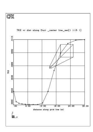
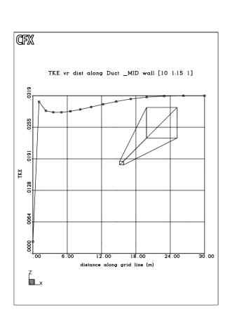
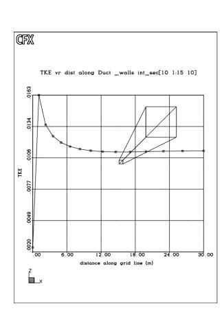
ducts. The starting point of this design effort is an experimental program performed by Liou and Wu [1] using the model shown in Figure 1. The aim of this work was to examine the complex flow present in the combustor, especially the turbulence, in order to provide data for use in validating CFD simulations and various turbulence models. The experimental model is a simplified example of a side-dump combustor chamber where air is used for both inlets flows i.e. a non-reacting flow. Long dimensions in the axial and transverse directions were chosen to generate a region of two-dimensional flow in the center of the model. Experimenters measured the mean flow field and turbulence intensity field throughout the combustor to determine the mixing efficiency for the case of perpendicular side inlets. Quantities measured included mean velocity and turbulence intensity components, Reynolds stresses and turbulent kinetic energy, or TKE. The measurement technique used to measure the flow field was LDV. This laser-based method measures the motion of small seeding particles, which move with the flow to estimate the mean flow properties. Variations in the mean velocity measurements are used to calculate the average turbulent velocity components The effective measurement volume of the laser method is between 1.84E-3[mm3] and 4.84E-3[mm3]. The seeding particles used in this experimental program were condensed saline solution droplets, which follow the flow closely and presumably have negligible effect on the fluid density and flow properties.
Side View All dimensions in mm Not to scale Figure 1. Experimental model of side-dump combustor. The test
geometries were non-dimensionalised as: X* = X / 15[mm] (X<0) ; X* = X / 30[mm] (X>0) ; Y* = Y / 15[mm] To allow the results to be more easily applied to similar geometries at different scales. The article lists the measurement and data processing error for the LDV method as up to 2.4% for the mean velocity components and up to 3.1% for the turbulence quantities. A mass conservation analysis based on the measured velocities was accurate within 4.25% with this variation attributed to slight inconsistencies in the fan flow rates. The experimental results have not been sufficiently verified and can therefore only be used as a guideline in validating the CFD results. B Flow description The mean flow velocity in the fully-developed section of the combustor was measured as 23.9[m/s]. the Reynolds numbers based on this reference speed and the height of the combustor is 45 600. the authors justify the use of a single Reynolds number to characterize the flow based on previous experimental work with no axial inlet stream present. These experiments demonstrated that the flow field is insensitive to changing Reynolds number in the range from 2 900 to 200 000. A Reynolds number of 45 600 indicates that the combustor flow is fully turbulent which means the difficulties in modeling transitional flow in CFD simulations can be avoided. The distance between the head plate and the upstream edge of the side inlets was chosen to be one half of the combustor height. This position was shown to maximize the amount of the side inlet flow pulled into the dome region (X* = -1 to X*=0) during preliminary tests without an axial inlet flow. This resulted in maximum mixing efficiency for this configuration. The combination of the high-speed axial flow and the two-side inlet flows form two main features of interest: twin counter-rotating vortices in the dome region and two separation bubbles downstream of the side inlets. The region between the two separation bubbles is equivalent to a nozzle through which the mean flow passes, undergoing a contraction and expansion in the process. Downstream of the separation bubbles the flow steadily becomes more fully developed. According to the data presented, uni-directional flow is achieved at approximately X*=4 and fully developed flow is present at X*=9. The average U-component of velocity at X*=9 is 25.04[m/s] with –6.7[%] maximum variation; the average V-component of velocity at this position is 0.037[m/s], or negligible compared to the axial flow. Liou and Wu state that the size of the separation bubbles and the position of the flow reattachment point are important parameters in validating various turbulence models applied to the flow. The reattachment position was experimentally determined to be at X*=1.2 and agrees well with visual methods. They also indicate that the high-speed axial flow possess enough momentum to maintain its width as it passes through the side inlet flows and therefore acts as a moving flat plate. The axial flow shifts the position of the vortices compared to the case where only side inlet flows and no axial flow are present. The high velocity gradients produced by the interaction of the axial and side inlet flow are a difficult test of turbulence models. The presence of the separation bubbles also demand the use of a turbulence model, which can handle complex flow geometries. The experimental model uses bell-mouth reducing sections to ensure that the flow profiles at the axial and side inlets are as uniform as possible. The side inlet average velocities are 19.74 and 19.45[m/s] with –1.1 and 0.7[%] maximum variation, respectively. The axial inlet average velocity is 92.73[m/s] with 0.6[%] maximum variation. All of these profiles can be considered uniform and form the basis for the modeled boundary conditions presented below. The experimental data shows that the mean and turbulent flow is generally symmetric about the combustor centerline, although significant non-symmetry occurs within the vortices and separation bubbles due to the flow reversals present. Turbulent kinetic energy is calculated from the experimental data as (3/4)[(u’) 2 + (v’) 2]. In this treatment the Reynolds shear stresses are proportional to both TKE and mean velocity gradients. Maximum levels of TKE are therefore found in areas of the flow where high velocity gradients lead to high shear stresses. However, non-zero TKE is measured at the combustor centerline even though symmetrical flow yields near-zero TKE is measured at the combustor centerline even though symmetrical flow yields near-zero mean velocity gradients because non-zero turbulent intensities are present. The distribution of turbulence in the experimental model is measured to be anisotropic and varies as the flow progresses down the combustor. Turbulent kinetic energy, or TKE, is initially introduced to the flow at the interface between the high-speed axial flow and the side inlet flows due to the high velocity gradients produced. Additional turbulence is produced by the shear stresses at the separation bubbles. As the mean flow expands through the virtual nozzle formed by the separation bubbles, TKE dissipates towards the walls of the combustor. By the time the flow is fully developed close to X*=9 the TKE has become virtually constant across the combustor. The turbulence past this point in the flow is very isotropic and comparable to the value experimentally measured in other rectangular ducts. The anisotropic nature of the turbulence field in this combustor model means that it is important to select a turbulence model for CFD simulations which properly handles this type of turbulence distribution. C Modeling goals The goal of the CFD modeling effort in this report is to develop CFD simulations to analyze the relative effect of side inlet angle on combustor mixing efficiency. Once a preliminary model has been developed with a perpendicular side inlet, it will be validated against the experimental results to the extent possible. This includes an evaluation of the suitability of the turbulence model used. Once a suitable accurate model has been designed, it will be modified to incorporate different side inlet angles. The results of these simulations will provide mixing efficiency data for an optimization analysis. The range of angles within 20 degrees of the perpendicular case is suggested as an appropriate optimization range. To simulate computational constraints, a maximum of 5000 elements will be used for the CFD simulations. The steps followed in performing a CFD analysis of the combustor flow are as follows:
3 Methodology A Simulation Setup I Flow domain selection The experimental model was designed to allow easy translation into a two-dimensional CFD model. For the CFD simulations here, an orthogonal grid with seven surfaces is proposed to discretise the model (Figure 2). This allows for simple definition of the axial inlet boundary condition and facilitates finer meshing across the axial flow.
All dimensions in mm Not to scale
The co-ordinate system used in the experimental program is duplicated in the CFD model to allow easier comparison between their results. Specifically, the origin of the co-ordinate system is placed on the combustor centerline in line with the upstream edge of the side inlet. The x-axis is aligned with the combustor centerline, the y-axis runs from the centerline to the wall of the combustor and the z-axis is places consistent with standard right-hand convention. The experimenters designed their model to produce a two-dimensional flow in the center plane. Measurements made in the z-direction show that the mean velocity components are uniform within 2.7[%]. This check was performed within the separation bubbles, which presumably would present the worst possible case to test the two-dimensional assumption. It can therefore be assumed that the model can be analyzed as a two-dimensional flow. In order to adapt our grid design to TASCflow’s three-dimensional solver, our grid is extruded 5[mm] in the positive z direction and two symmetry planes are applied to
maintain the flow as two-dimensional. As noted above, the combustor flow becomes fully developed after the X*=9 plane with minimal variation in the axial velocity. The grid design is therefore truncated at this position in order to use the fixed number of elements efficiently. Elements, which are not needed to resolve the fully developed flow can then be used to better, calculate the more complex flow in the dome region. Symmetry across the combustor centerline is also implemented to eliminate redundant elements and increase mesh efficiency. The working fluid used in all models was air at standard conditions. The default property values of ρ= 1.164[kg/m3] and μ = 1.824E-5 [N-s/m2] already present in TASCflow were used. SI units were used to maintain similarity with the experimental data. II Boundary conditions The boundary conditions used in the CFD model are summarized in Table 1. the values for the flow parameters of the two inlet planes are roughly the average values. As shown above the inlet velocity profiles are fairly uniform with minimal variation. It is also noted that the transverse flow at each plane is negligible compared to the normal flow across the plane. We can therefore model each as a steady, constant velocity normal to the inlet boundary plane. The outlet boundary condition is specified as a constant velocity plane. Although there is a slight variation in the experimentally measured velocities at this position (X*=9), it is sufficiently uniform to be modeled as a constant, steady outflow. the alternative is to proscribe a constant pressure plane at the outlet. However, this condition is not physically consistent with the flow in question since a fan on the outlet of the experimental model produces a negative pressure in the combustor relative to ambient. This pressure is not specified in the experimental results, so a velocity outlet condition is selected instead. Three symmetry planes and a composite wall boundary condition are also specified. The wall prevents mass transfer across the five surfaces while the symmetry planes prevent gradients from forming across them. The three symmetry planes were specified independently because it was not clear whether combining them into a single composite plane would be physically valid in the CFD software.
Figure 3. Boundary conditions for CFD simulations.
Table 1. Summary of boundary conditions for CFD simulations.
III Grid design This section require direct contact. [thank you for your interest] References [1] T.M. Liou, Y.Y. Wu. 1992. LDV measurements of the flowfield in a simulated combustor with axial and side inlets. Experimental Thermal and Fluid Science, Vol. 5, pp. 401-409. [2] Darkos, N. 1997. CFX-TASCflow User Documentation. [3] Laser Doppler anemometry www.dantecmt.com [4] Principles of laser Doppler |
|||||||||||||||||||||||||||||||||||||||||||||||||||||||||